LLM Inference: Insights into Memory and Performance
Generating content with Large Languge Models (LLMs) depends on two steps: training, where models learn from vast datasets, and inference, where they apply the knowledge to produce responses.
Training builds the brain; inference makes it talk, fast and scale. The catch? Fitting massive models into memory and handling thousands of users is no small feat.
This post dives into the details of LLM inference, focusing on memory management for VRAM, performance metrics such as latency and tokens per second (TPS) and the role of GPU capabilities in optimizing large-scale deployments.
Here’s your guide to the key points.
Theoretical Memory Calculation for LLMs
Using an LLM on a GPU depends on handling its VRAM, shown in this formula:

- Model Memory: Space allocated for the model’s weights.
- KV Cache: Saves the “key” and “value” results from past tokens. Think of it as keeping notes from earlier steps so the model can work faster.
- GPU Overhead: It’s like the GPU’s own workspace, stuff it keeps for running smoothly, not for the model’s weights or its calculations.
To better understand how these components interact and impact LLM inference, let’s dive deeper into each one.
Model Memory
Model Memory refers to the space allocated for storing the model’s weights, which are the core parameters learned during training.
These weights determine how the model processes input data and generates outputs. The size of the model memory depends on the number of parameters in the LLM and the precision format used (e.g., FP16, INT8, or INT4).
For example, a model with billions of parameters can consume hundreds of gigabytes of VRAM in its raw form, but quantization can significantly reduce this footprint.
Quantization is a technique that enables LLMs to use less VRAM/RAM and operate faster. It reduces memory consumption and increases processing speed by converting the model’s weights and computations from higher precision formats like 16-bit (FP16) or 32-bit (FP32) to lower precision formats such as 8-bit (INT8), 4-bit (INT4), or even lower levels (INT2, INT1).
While quantization can lead to a reduction in model accuracy, advanced quantization techniques like GPTQ and AWQ help minimize this loss.
The memory required to store the model’s weights can be calculated using the following formula:

- P: Number of model parameters
- 4B: 4 Bytes per parameter
- Q: Quantization (in bits)
For a model like Llama 8B with FP32 precision, the memory required for the weights can be calculated as follows:

KV Cache
Key-Value Caching is a technique in transformer models where the key and value matrices from previous steps are stored and reused during the generation of subsequent tokens. This means that instead of recalculating all past tokens every time a new token is generated, the model retrieves the previous computations from the KV Cache.

- B: Batch Size is the number of sequences processed simultaneously. Increasing the batch size increases the memory required for the KV Cache because the model needs to store key-value pairs for all sequences in the batch.
- S: Sequence length is the number of tokens in the input sequence. Longer sequences require more memory because the KV Cache stores key-value pairs for every token in the sequence.
- L: Number of layers is the number of transformer layers in the model. Each layer has its own set of key-value pairs, so the memory scales with the number of layers.
- H: Hidden size is the dimensionality of the hidden states (key and value vectors). Larger hidden sizes increase memory usage because each key and value vector is larger.
- P: Precision is the number of bytes used to store each parameter (e.g., FP16 = 2 bytes, FP32 = 4 bytes). Lower precision (e.g., FP16) reduces memory usage but may affect model accuracy.
Each token generates both a key and a value, so the memory requirement is doubled. For example:
- Batch Size (B): 1
- Sequence Length (S): 2048
- Number of Layers (L): 32
- Hidden Size (H): 4096
- Precision (P): 1 byte (INT8)
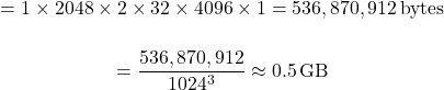
The formula highlights how KV Cache memory usage scales with batch size, sequence length, and model architecture, enabling better planning for large-scale deployments.
GPU Overhead
GPU overhead refers to the additional memory and resources required by the GPU to manage tasks beyond just storing the model’s weights and KV Cache. It includes:
- Intermediate Activations: Temporary storage for activations during forward and backward passes.
- CUDA Kernels: Memory for GPU kernels and their execution.
- System Overhead: Memory reserved by the GPU driver and runtime for managing tasks.
- Workspace Memory: Memory used for optimizations like cuBLAS or cuDNN operations.
Unlike Model Memory and KV Cache Memory, GPU overhead is not directly tied to the model’s architecture but depends on the GPU hardware, drivers, and the deep learning framework being used.
GPU overhead is typically 5–10% of the total VRAM but can vary depending on:
- GPU Architecture: Newer GPUs have better memory management and lower overhead.
- Framework: PyTorch, TensorFlow and other frameworks have different overheads.
- Workload: Complex operations (e.g., attention mechanisms) increase overhead.
Performance Metrics
When deploying large language models (LLMs) in real-world applications, understanding and optimizing performance metrics is crucial. These metrics not only determine how efficiently a model operates but also directly impact user experience and system scalability. Whether you’re serving a chatbot, a translation service, or a content generation tool, three key metrics stand out: tokens per second (TPS), latency and max concurrent users.
TPS (Tokens per Second)
TPS measures the number of tokens a model can generate per second. It is a key metric for evaluating the inference speed of a model. The TPS value can be estimated using the GPU’s processing capacity (FLOPs/s) and the model’s computational requirements per token (FLOPs/token):

- GPU FLOPs/s: The theoretical computational power of the GPU (Floating Point Operations per Second).
- Model FLOPs/token: The number of floating-point operations required to generate one token (depends on the model’s size and architecture).
- Efficiency Factor: Typically ranges between 0.3 - 0.6 accounting for real-world inefficiencies.
In real-world scenarios, the theoretical TPS value is significantly reduced due to factors such as:
- Memory bandwidth limitations
- Cache optimization inefficiencies
- Quantization (4-bit, 8-bit, 16-bit)
- Parallelization efficiency
Latency
Latency is the time delay between a user sending a query and receiving a response. It is a critical metric for user experience.
- Low Latency: Faster responses, better user experience.
- High Latency: Users experience delays, and the system may become congested.
- Latency Response: The total time for the user to receive a complete response.

The latency can be broken down into two components:
- Latency per Token: The time the model takes to generate one token.
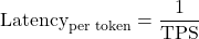
- Avg Tokens per Request: The average number of tokens generated per user request.
Max Concurrent Users
The maximum number of concurrent users a system can handle depends on the total TPS, response time, and average tokens per request.

To increase the number of concurrent users:
- Increase TPS: Use more powerful GPUs or optimize the model (e.g., FP16, quantization).
- Reduce Response Time: Improve first-token latency and inference speed.
- Reduce Avg Tokens per Request: Generate fewer tokens per user request to serve more users simultaneously.
Efficiently deploying LLMs requires balancing memory usage, inference speed, and scalability. By understanding and optimizing these key factors, you can ensure your models deliver fast, reliable, and cost-effective performance in real-world applications.
As the field of AI continues to evolve, staying ahead of the curve requires a deep understanding of these foundational concepts. Whether you’re deploying a small-scale application or a large-scale service, the principles outlined in this post will help you make informed decisions and build systems that stand the test of time.
Thank you for reading!